
On this page

When a business runs on several public clouds, in several regions, and inside different compliance boundaries, the "pull everything back to a central cluster and analyze it there" approach to observability hits four problems. Cross-cloud network costs grow with data volume. Cross-cloud queries slow down incident response. Some raw data is not allowed to leave its region. And the central cluster itself becomes a performance bottleneck and a single point of failure.
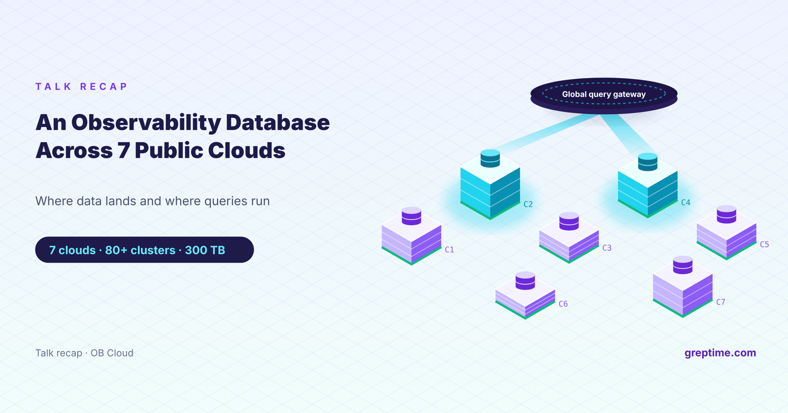
This article uses OceanBase Cloud (OB Cloud) as a production reference and looks at how to design an observability database for multi-cloud environments: where data is written, where queries execute, how object storage becomes part of the database, and how the system meets cost, performance, autonomy, and consistent-experience requirements at the same time. Our conclusion: a multi-cloud architecture should manage data that stays distributed across clouds, give users one consistent experience, and keep each cloud's cluster autonomous. It does not need to move all data into one place.
OB Cloud: production on seven clouds
OB Cloud has offered an integrated multi-cloud database service since 2022. It covers 7 major public clouds, 16 countries and regions, 60+ regions, and 240+ availability zones, with cross-region and cross-cloud disaster recovery.
A cloud database that promises a consistent experience needs observability deployed alongside it in every cloud. Logs cannot leave their region freely because of compliance rules, and engineers cannot be expected to troubleshoot by switching between seven unconnected tools.
Four kinds of logs, one conflict
OB Cloud handles application logs, OBServer logs, OBProxy logs, and SQL Audit logs. The four differ in write volume, schema, retention, and query patterns, yet incident investigation needs to correlate them.
In OB Cloud's production experience, about 95% of these logs are never queried. When an incident happens, though, engineers need to search hours or even days of data immediately. Storage has to stay cheap most of the time, and the few useful records have to be found fast when something breaks.
Every new cloud means another adapter
The logging services of Alibaba Cloud, Huawei Cloud, Tencent Cloud, Baidu AI Cloud, AWS, Azure, and Google Cloud differ in collection agents, query languages, identity and access, and object storage interfaces:
| Cloud logging service | Typical agent | Query language |
|---|---|---|
| Alibaba Cloud SLS | Logtail / LoongCollector | Lucene + SQL |
| Huawei Cloud LTS | ICAgent | Lucene-like |
| Tencent Cloud CLS | LogListener | Lucene-like |
| Baidu Cloud BLS | LogAgent | Lucene-like + SQL |
| AWS CloudWatch | CloudWatch Agent | Logs Insights |
| Azure Monitor | Azure Monitor Agent | KQL |
| GCP Logging | Ops Agent / Fluent Bit | Logging Query Language |
An observability platform built directly on these services has to write a new adapter for every cloud it adds. A unified API layered over seven query languages is just as expensive to maintain over time.
First generation: Loki cut storage cost but limited queries to minutes
OB Cloud's first-generation design used Grafana Loki: label indexes plus object storage. Storage cost dropped, and Loki plugged straight into Grafana. Loki indexes labels only, not log content. Keyword searches over log bodies had to scan large amounts of data and often timed out, so the log viewer's default query window had to be set to a few minutes.
With logs that are rarely read but must be searchable the moment something fails, the bottleneck moved from the collection pipeline to the database, which has to trade off low-cost storage against fast retrieval.
After moving to GreptimeDB
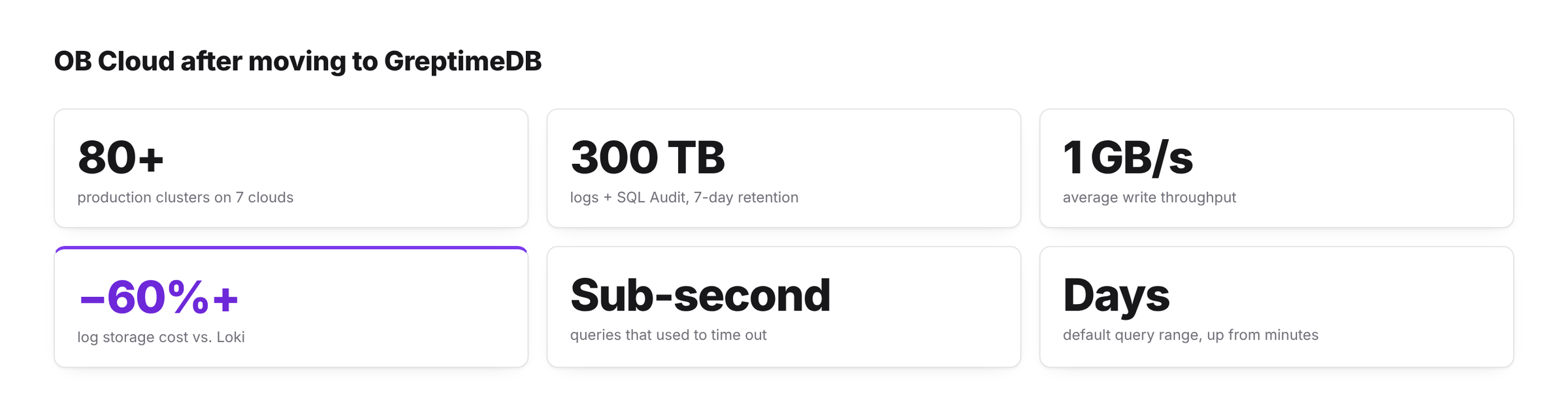
After the migration to GreptimeDB, OB Cloud runs 80+ production clusters across 7 public clouds. Under a 7-day retention period they hold more than 300 TB of log and SQL Audit data; the largest single cluster holds 50 TB, and average write throughput is about 1 GB/s. Compared with the previous Loki setup, overall log storage cost fell by more than 60%. Queries that used to time out now return in sub-second to single-second latency, and the default query range grew from minutes to hours and days.
The full migration story is in the OB Cloud case study.
Issues surfaced by real workloads drove several rounds of GreptimeDB improvements during the migration:
- v0.15 added Pipeline filtering by log level and keyword, so unneeded logs are dropped at ingest;
- v0.13 introduced a new full-text index implementation and query functions, making queries simpler and faster;
- v0.15 changed the Compaction file-merge strategy to lower peak memory during merges, fixing Datanode OOMs under heavy writes;
- v0.15 made Metasrv fully support RDS as the metadata store and shipped a migration tool, so OB Cloud no longer runs a separate etcd;
- GreptimeDB Enterprise auto-scaling, auto-partitioning, load balancing, tiered caching, and intelligent flow control went into production.
Beyond logs, OB Cloud is now switching the SkyWalking backend storage to GreptimeDB, so that trace and APM data are stored and processed in the same system as logs and made available to its SRE agent. It currently uses a SkyWalking fork with GreptimeDB storage support: killme2008/skywalking.
Multi-cloud changes the data boundary and the query boundary
Any multi-cloud system that continuously produces high-throughput observability data runs into the same five bottlenecks as OB Cloud:
- Cross-cloud transfer is expensive. Moving high-throughput data across clouds over long periods drives up both network cost and transfer time.
- Remote centralized queries are slow. Every cross-cloud round trip adds to time spent on an incident.
- Data residency and compliance limit movement. Data sovereignty rules may forbid raw logs from leaving a location or region.
- A single center carries too much load and risk. One center handling all writes and queries is both a performance bottleneck and a single point of failure.
- Cloud infrastructure differs. Object storage APIs, networking, IAM, and Kubernetes environments are not identical, so a deployment cannot be copied as-is.
Multi-cloud observability therefore has to drop the "pull everything to the center" assumption and redraw two boundaries: how far raw data is allowed to move, and at which layer queries are completed.
Architecture: logically unified, physically distributed
A multi-cloud observability database has three layers: a global layer, a cluster in each cloud, and a storage plane. The design work is in defining each layer's responsibilities and failure boundary, without a single control plane spanning every cloud.
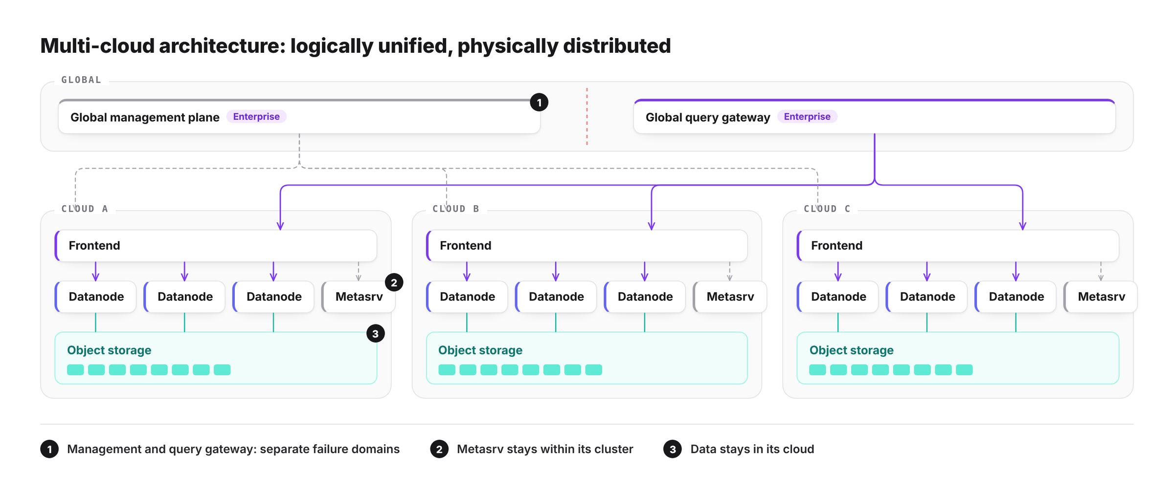
| Layer | Responsibilities | Boundary |
|---|---|---|
| Global management plane | Tenants, quotas, access logs, cluster lifecycle, unified operations entry point | Enterprise feature; a separate failure domain from the global query gateway |
| Global query gateway | Unified query entry point, cross-cloud routing, result merging | Enterprise feature; does not replace in-cloud query planning |
| Per-cloud GreptimeDB cluster | Local writes, queries, metadata, and routing | Fully autonomous; Metasrv manages only its own cluster and never spans clouds |
| Storage plane | Hot, warm, and cold data with indexes, lifecycle, and location metadata | Data stays in its own cloud and compliance region where possible |
Inside each cluster, GreptimeDB keeps its usual division of roles: Frontend handles protocol endpoints, query planning, and result aggregation; Datanode scans data and prunes with indexes; Metasrv maintains metadata and routing. Each cloud runs a complete cluster that is physically isolated and operates independently. The global layer provides only the unified management and access entry points.
Storage tiered by temperature
- Hot data sits on local SSDs, cloud disks, or a cache layer for low-latency access.
- Warm data sits on object storage such as S3, OSS, COS, GCS, ABS, MinIO, or HDFS, with indexes keeping query cost under control.
- Cold data moves to archive storage or infrequent-access object storage for cheap long-term retention.
- Metadata records Regions, files, indexes, time ranges, lifecycle, and data location, and drives query pruning and routing.
From decoupled compute and storage to compute-compute separation
A traditional shared-nothing architecture binds storage and compute to the same nodes. Resources can only be allocated coarsely, and scaling usually means moving data. GreptimeDB first moves persistent data to object storage, turning Frontend and Datanode into an elastically scalable compute layer. It then splits compute by workload: writes, online queries, large-scale analysis, and historical queries run on Datanodes with different roles.
This gives finer-grained isolation. Write spikes do not slow down online queries, and large analytical scans do not take compute away from live troubleshooting.
Write path: WAL and WAL-less
Writes first reach the local Frontend, which identifies the tenant, routes to shards, and batches adaptively. Once a batch is formed, the system takes one of two paths depending on the workload:
- Standard WAL path: data goes to the WAL and the Memtable, then is flushed to object storage. Suited to workloads that need low-latency acknowledgment and general recovery semantics.
- Enterprise WAL-less path: Frontend aggregates small writes into large batches suited to columnar storage and writes them straight to object storage, skipping a WAL write and the associated service cost. Intended for sustained, very high throughput.
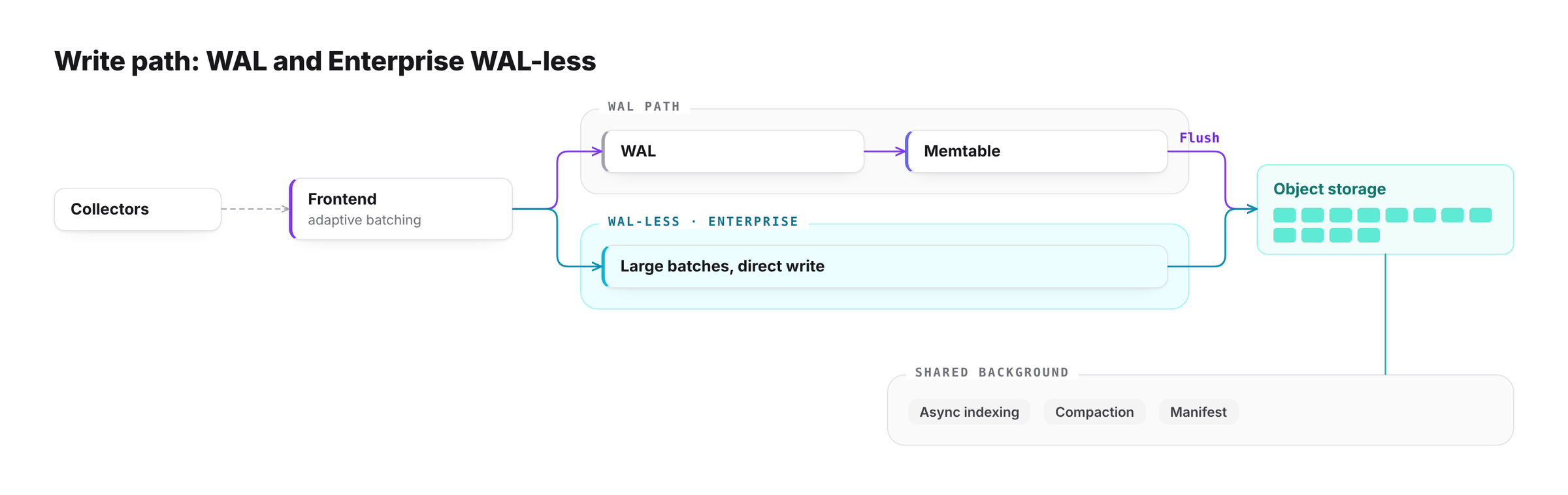
Both paths share async index building, Compaction, and Manifest management afterwards. WAL-less is meant only for sustained, very high-throughput workloads: it depends more directly on object storage availability and must be paired with backpressure, buffering, and capacity control. When object storage has problems, the WAL path can buffer briefly in the WAL and Memtable, while the WAL-less path has to apply backpressure sooner.
Four properties of object storage
Object storage makes capacity and cost more elastic, but it behaves very differently from a local file system:
- Latency is higher, and every GET or PUT request is billed;
- Changing a key or path usually means copy-then-delete; there is no cheap rename;
- Uploads mostly overwrite whole objects; you cannot modify data in place the way you can on a local disk;
- LIST is expensive and returns a limited number of entries per call, so directory listing cannot serve as a metadata system.
Object storage lowers media cost and shifts complexity into the write, cache, metadata, and query scheduling layers. The database has to deal with these differences itself.
Writes go through a local write-back cache; reads go through IO scheduling
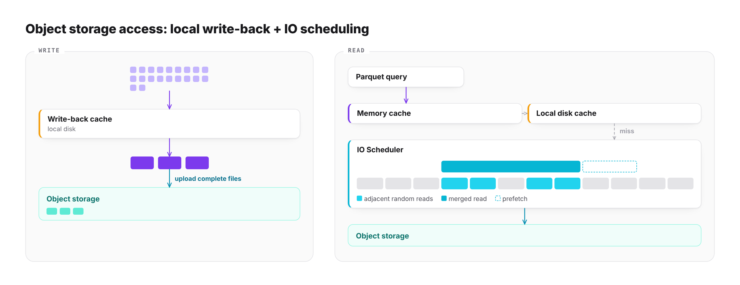
On the write side, data is first written in full to a local write-back cache, so the hot path completes locally. Background tasks then upload complete files to object storage in batches. Multipart upload is one of the upload mechanisms; the reduction in API calls comes mainly from the write-back cache merging many small writes into fewer, larger objects.
On the read side, Parquet queries against object storage often turn into many small, adjacent random reads. The IO Scheduler recognizes how these requests sit relative to each other, merges adjacent random IO into larger sequential reads, and prefetches data blocks and metadata likely to be needed next based on Parquet access patterns. Memory and local-disk caches hold hot data, indexes, and metadata, cutting the number of remote requests and raising effective throughput.
Opening data through Iceberg
Data in object storage should also be usable by other compute engines. The Enterprise Iceberg exporter reads statistics from tables, Regions, the Manifest, and Parquet footers, and generates standard Iceberg metadata. Iceberg DataFiles point directly at GreptimeDB's existing Parquet files, so no data is copied.
On the same underlying data, GreptimeDB keeps handling real-time writes and online queries, while engines such as Spark and Trino read it for offline analysis, data processing, or AI workloads. Adding or replacing a compute engine later does not require migrating existing data.
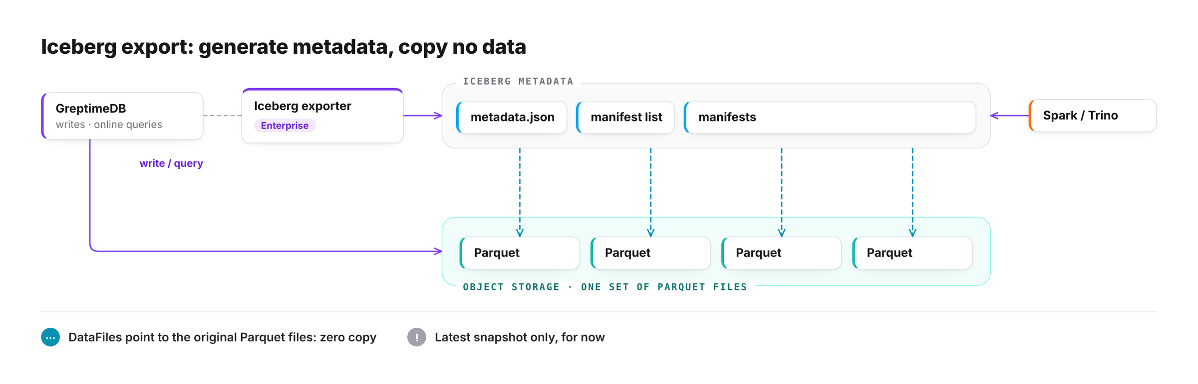
Currently the integration supports reading the latest snapshot only; full schema history and time travel are still in development. Regular tables, Dense metric tables, and Sparse metric physical tables use different export layouts, so check the mapping rules for your version before using them from an external engine.
Query performance: tiered indexes and two-level pruning
Spend the index budget by data value
Log queries typically combine a time range, service or instance filters, keyword search, structured field filters, aggregations, and context lookups. Building full-text indexes on every field for all data makes index cost grow faster than query benefit.
We build indexes in tiers:
- Time index: present on all data and used for basic range pruning.
- Tag index: covers frequently filtered dimensions such as service, host, namespace, and pod.
- Field statistics: low-cost statistics such as MinMax, ZoneMap, and NDV narrow the range quickly.
- Bloom filter: quickly rules out data blocks that definitely do not contain the target value.
- Inverted and full-text indexes: enabled only for key fields, hot data, or high-value tenants.
- Columnar storage and statistics: serve structured filtering and aggregation.
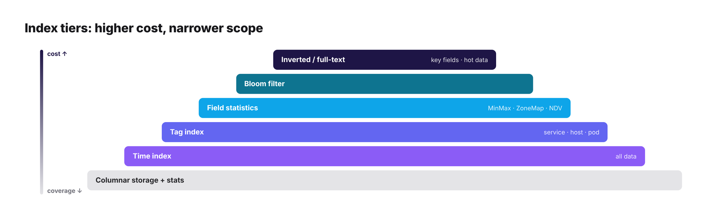
The goal is to make the most common and most important troubleshooting queries fast enough while keeping index cost under control.
OB Cloud's log table is a concrete example: the message field has a full-text index for keyword search, the high-cardinality request_id uses a skipping index for point lookups, and the remaining fields have no index to keep storage cost down.
Cross-cloud queries must avoid broadcast
Broadcasting a query to every cloud, scanning, and then merging multiplies both cost and latency. Our query path prunes at two levels:
- The global query gateway receives the request and narrows it to the relevant clouds based on tenant, time range, the global catalog, and data residency rules. Clouds that do not match receive no request.
- Inside each target cluster, Frontend plans the query and locates the relevant Regions using routing information from Metasrv; Datanodes then prune at the file, data block, and index level.
- Filters and partial aggregations are pushed down to where the data lives, and each cloud returns only matching rows or partial aggregates.
- The global query gateway performs the final merge, sort, limit, and aggregate combination.
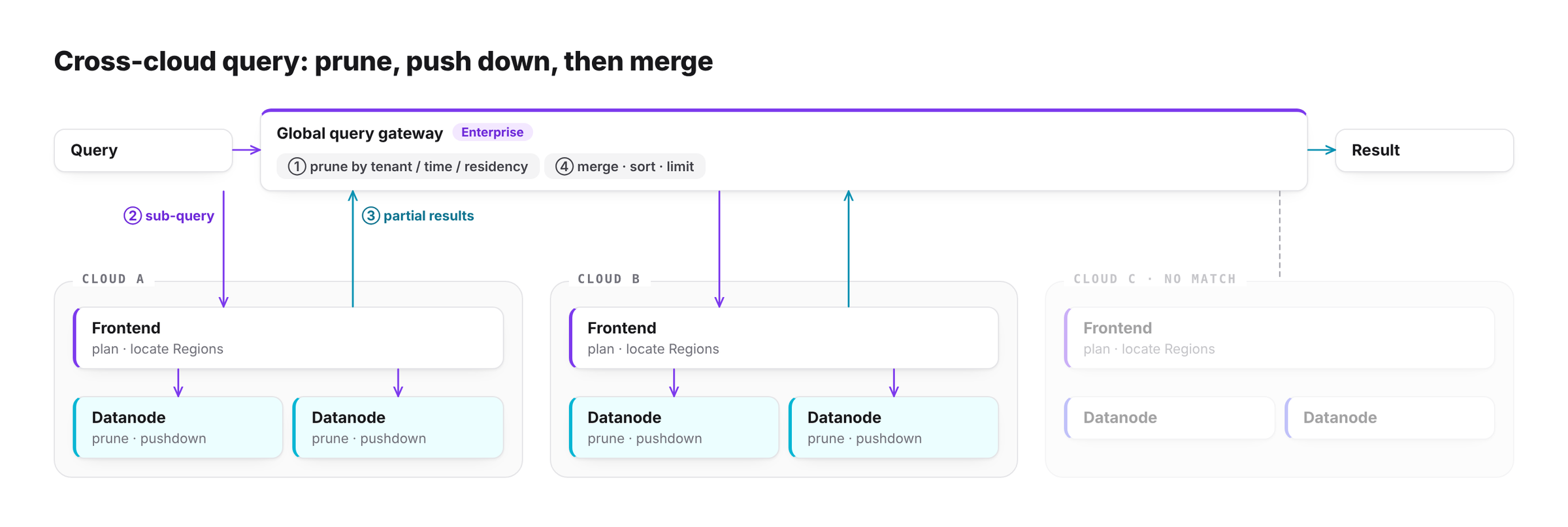
The responsibility boundary has to stay clear: federated cross-cloud queries belong to the global query gateway, and Metasrv handles metadata and routing only within its own cluster.
Long-term governance of a multi-cloud system
Multi-tenant isolation
A multi-tenant environment needs at least six kinds of isolation: tenant-level data isolation; write quotas and rate limits; query concurrency and resource queues; index budgets and field-level policies; retention and lifecycle; and permissions, access logging, and encryption.
The Enterprise Workload abstraction first pools shared resources, then uses the Workload as the unit for pricing, capacity limits, flow control, and autoscaling decisions. QuotaCenter is designed around three requirements: a QuotaCenter failure must not affect user requests; quota checks must not block requests; and callers must not be able to bypass quotas by splitting a large request into many small ones.
Layered failure handling and degradation
| Failure | Expected degradation |
|---|---|
| Global management plane down | Per-cloud clusters keep serving independently |
| Global query gateway down | Cross-cloud queries are unavailable; each cloud's local entry point keeps serving |
| Metasrv down within a cluster | While cached routes remain valid, existing Regions can keep serving reads and writes for a short time; DDL, route changes, and failover are restricted |
| Object storage failure | The WAL path can buffer briefly and applies backpressure once it cannot flush; WAL-less depends more directly on object storage and has to throttle sooner |
| Network partition between clouds | Local clusters keep serving; once the network recovers, the global catalog and runtime state resynchronize |
| System under heavy load | Pause low-priority Compaction, limit large queries on cold data, and prioritize hot data and critical tenants |
Each layer must specify which capabilities it can still provide on its own when the layer above fails, how long it can sustain them, and when it must apply backpressure or reject requests. Reliability is made up of this set of degradation paths and their preconditions.
Cost governance
- Tenant and signal quotas: attribute write, storage, query, and index cost to tenants and signal types, and set budgets and quotas for each.
- Data lifecycle: set retention periods, sampling rates, and hot/cold tiering per cloud, tenant, and compliance region.
- Query behavior statistics: track scanned volume, cross-cloud transfer, and cache hit rate per query, then use query profiles to tune caching, pruning rules, indexes, and data layout.
A migration can validate the architecture. As scale keeps growing, ongoing governance keeps every cost attributable, predictable, and optimizable.
Toward Observability 2.0
Once logs, metrics, and traces live in the same columnar storage on object storage, they can be treated as one kind of data: timestamped events. Metrics, logs, and traces are three views over the same set of wide events.
json
{
  "timestamp": 1689024000,
  "host": "web-01",
  "service": "payment-api",
  "cpu_usage": 85.4,
  "level": "ERROR",
  "message": "Connection timeout",
  "trace_id": "a1b2c3d4e5f6",
  "duration_ms": 1540
}
The same events can be aggregated by host into a metrics view, searched by error level as logs, or used to reconstruct a call chain by trace_id:
sql
-- Metrics view
SELECT host, avg(cpu_usage) FROM events GROUP BY host;

-- Logs view
SELECT timestamp, message FROM events WHERE level = 'ERROR';

-- Traces view
SELECT trace_id, duration_ms FROM events WHERE service = 'payment-api';
Unification here means unified event semantics and derivable views. It does not require putting all data physically into one table. Flow Engine handles continuous aggregation, and Logs Engine handles log parsing, cleaning, and structuring.
Agents and observability are changing each other
On one side, an agent reads metrics, logs, and events, forms root-cause hypotheses with an LLM, verifies them with tools such as profiling, and then proposes a fix. The requirement is that every conclusion is backed by query and diagnostic evidence.
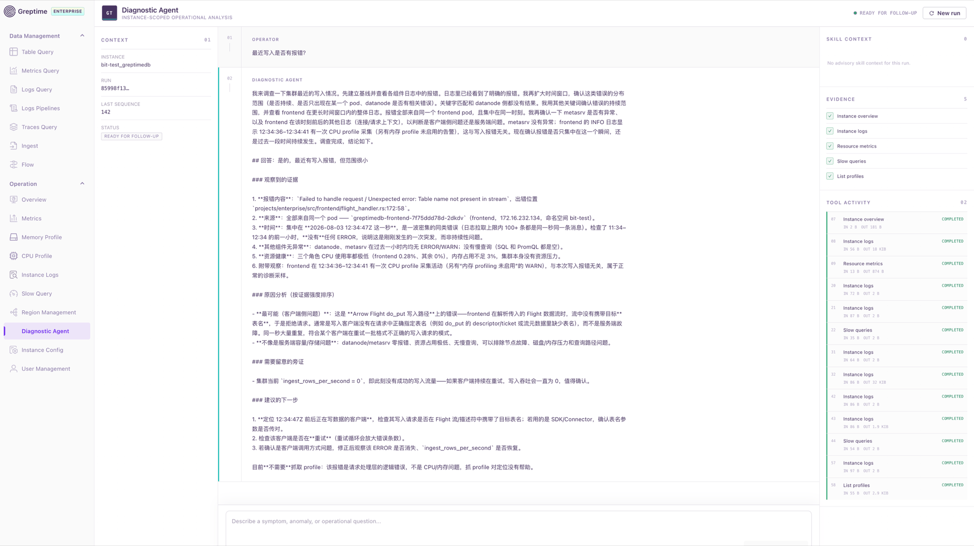
The screenshot shows one run of the GreptimeDB Enterprise Diagnostic Agent (preview); the question and the answer in this run are in Chinese. The user asks whether there have been any recent write errors. The agent checks the instance overview, component logs, resource metrics, slow queries, and the profile list, and establishes that the errors all come from one Frontend pod, are concentrated within a single second, and that no other component shows problems. It concludes that a client sent write requests without a table name, and states that no profile capture is needed this time.
On the other side, observability systems need to give agents machine-readable semantics. The Table Semantic Layer (experimental) stores signal type, source, metric type, unit, temporality, and similar information. MCP Server and agents read it instead of guessing table names, fields, units, and aggregation methods.
Access patterns are changing too. A person troubleshooting usually follows one hypothesis deep. An agent is more likely to keep several candidate explanations open at once, query multiple signals, instances, and time windows in parallel, and then rule options out based on evidence. This means higher fan-out and denser bursts of small queries for the database, and new requirements for query budgets, cancellation, concurrency scheduling, caching, pruning, and cross-signal correlation.
Conclusion
For an observability database in a multi-cloud environment, our design puts management and access entry points in a global layer and keeps data and compute in each cloud's cluster. Object storage lowers long-term cost, while the write, cache, and query scheduling layers handle object storage latency, billing, and interface limits. Indexes are tiered by budget. Cross-cloud queries prune first and then push down. Every layer has defined degradation behavior when the layer above fails. OB Cloud started with logs and is now moving SkyWalking trace and APM data onto the same data foundation for its SRE agent; that foundation is also being prepared for higher-concurrency, semantics-driven agent queries.


