How do you switch an application from InfluxDB to GreptimeDB? This article walks through the full path.

If you're still weighing the switch on performance grounds, the GreptimeDB vs. InfluxDB benchmark report compares write and query throughput on the TSBS CPU workload.

The first thing InfluxDB users notice when migrating to GreptimeDB is protocol compatibility: GreptimeDB supports the InfluxDB line protocol, so many write paths only need a new URL, credentials, and database name. What actually determines migration quality, though, usually comes later: importing historical data smoothly, and rewriting existing InfluxQL queries as GreptimeDB SQL.

This guide breaks the migration into four stages. Stage 1 uses the TSBS IoT use case to build a dataset that resembles a real connected-vehicle workload, purely to make the later stages reproducible. If you already have your own InfluxDB data and queries, skip Stage 1 and start from the write migration or the historical data migration.

1. Prepare demo data (optional): write the TSBS IoT dataset into InfluxDB.

2. Migrate write requests: switch live writes from InfluxDB to GreptimeDB.

3. Migrate historical data: import existing line protocol data from InfluxDB into GreptimeDB.

4. Migrate InfluxQL: rewrite the TSBS IoT queries as GreptimeDB SQL, using GreptimeDB's range query where it fits.

The official documentation also has a more general InfluxDB migration guide and a range query reference. This article puts those capabilities to work in one end-to-end migration scenario.

Check the data model before you migrate

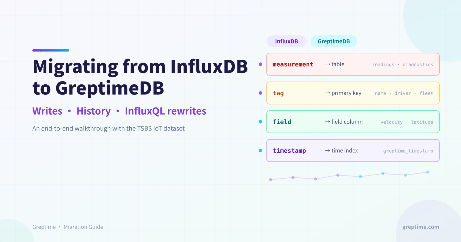
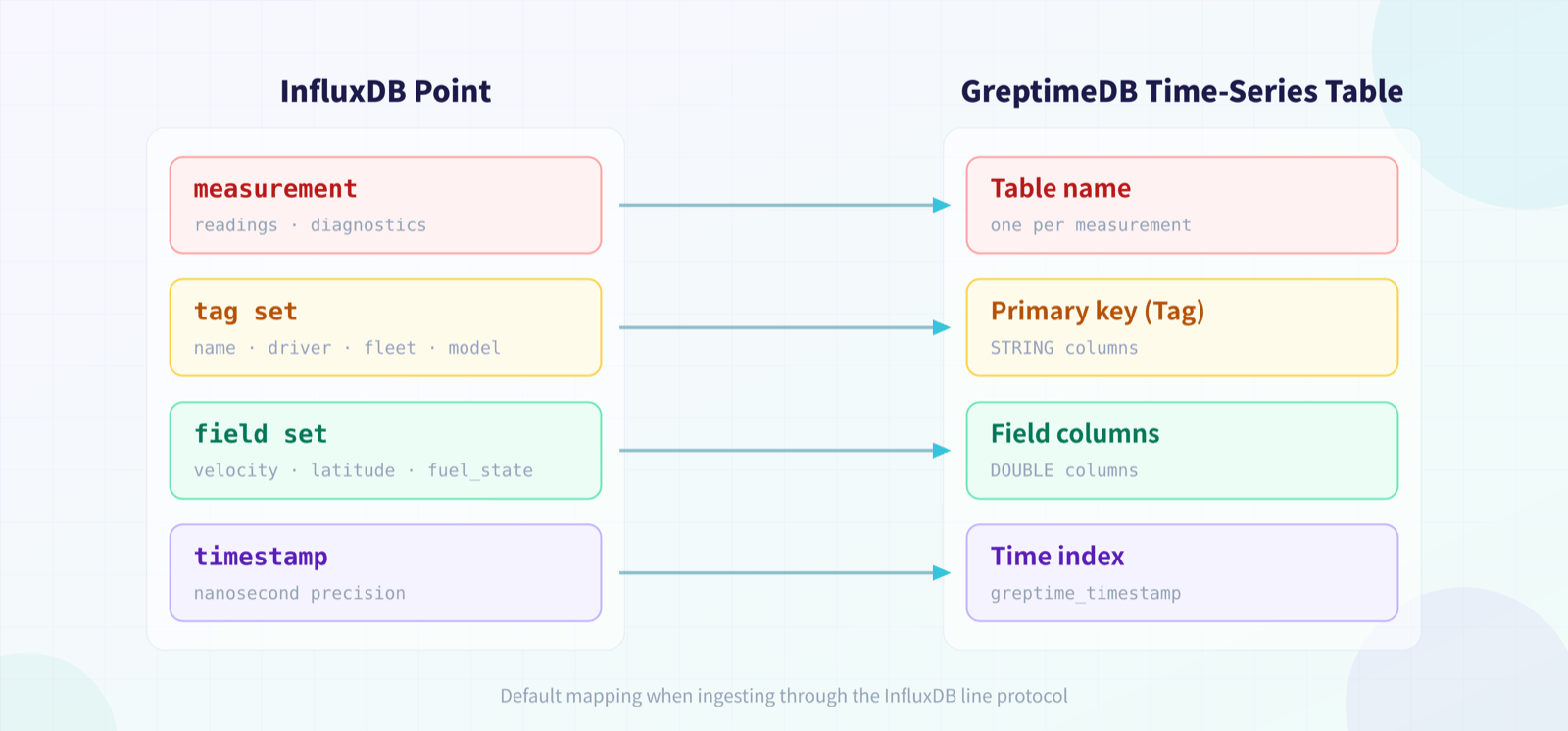
An InfluxDB point consists of a measurement, a tag set, a field set, and a timestamp. When you write it to GreptimeDB through the InfluxDB line protocol, GreptimeDB maps it onto a time-series table:

• The measurement becomes the table name, such as readings or diagnostics.

• Tags become primary key columns, such as name, driver, fleet, and model in TSBS IoT.

• Fields become regular field columns, such as latitude, longitude, velocity, fuel_state, and current_load.

• The timestamp becomes greptime_timestamp, a TimestampNanosecond column that is also the time index.

Default mapping from an InfluxDB point to a GreptimeDB time-series table

This means query migration doesn't have to treat measurements, tags, and fields as special concepts; they are already ordinary SQL tables and columns. After migrating, start by running:

DESC TABLE readings;
DESC TABLE diagnostics;
SHOW CREATE TABLE readings;
SHOW CREATE TABLE diagnostics;

If you created tables manually before migrating, you can name the time column ts or anything else. The SQL in the rest of this article assumes the default time column greptime_timestamp created automatically by line protocol ingestion.

1. Prepare demo data (optional)

This stage only exists to give the write migration, historical data migration, and query rewrites a reproducible dataset. If you already have an InfluxDB instance, line protocol data, or real production queries, skip to Stage 2.

Start a local InfluxDB 1.8 instance. This article uses the InfluxDB 1.x database model, which makes it easy to demonstrate the migration with TSBS-generated InfluxDB line protocol data and InfluxQL queries.

docker run --rm --name influxdb-1-8 \
  -p 8086:8086 \
  influxdb:1.8

Install TSBS. The TSBS repository ships several commands; this article needs tsbs_generate_data to generate data, and you can also use tsbs_generate_queries to generate sample InfluxQL queries.

git clone https://github.com/timescale/tsbs.git
cd tsbs
make

Generate InfluxDB line protocol data for the IoT use case. The scale below works for a local demo; for production load testing, increase --scale and widen the time range.

./bin/tsbs_generate_data \
  --use-case="iot" \
  --seed=123 \
  --scale=100 \
  --timestamp-start="2026-01-01T00:00:00Z" \
  --timestamp-end="2026-01-02T00:00:00Z" \
  --log-interval="10s" \
  --format="influx" \
  | gzip > tsbs-iot-influx.gz

Create the InfluxDB database and write the data. TSBS outputs line protocol, which goes straight into InfluxDB's /write API. To keep individual requests small, split the file by lines first.

curl -sS -XPOST "http://localhost:8086/query" \
  --data-urlencode "q=CREATE DATABASE benchmark"

mkdir -p tsbs-iot-parts
gunzip -c tsbs-iot-influx.gz \
  | split -l 5000 - ./tsbs-iot-parts/data.

for file in ./tsbs-iot-parts/data.*; do
  curl -sS -XPOST "http://localhost:8086/write?db=benchmark&precision=ns" \
    --data-binary @"${file}"
done

A quick check:

curl -G "http://localhost:8086/query" \
  --data-urlencode "db=benchmark" \
  --data-urlencode "q=SHOW MEASUREMENTS"

curl -G "http://localhost:8086/query" \
  --data-urlencode "db=benchmark" \
  --data-urlencode "q=SELECT count(*) FROM readings"

TSBS IoT typically generates two core measurements:

• readings: operational readings such as vehicle position, velocity, and fuel consumption.

• diagnostics: diagnostic data such as vehicle status, fuel state, and current load.

2. Migrate write requests

The core of the live write migration is pointing the InfluxDB write endpoint at GreptimeDB. GreptimeDB supports both the InfluxDB line protocol v1 and v2 write APIs.

First, start GreptimeDB. The command below runs a standalone GreptimeDB in Docker for this walkthrough:

docker run -p 0.0.0.0:4000-4003:4000-4003 \
  -v "$(pwd)/greptimedb_data:/greptimedb_data" \
  --name greptime --rm \
  greptime/greptimedb:v1.0.2 standalone start \
  --http-addr 0.0.0.0:4000 \
  --rpc-bind-addr 0.0.0.0:4001 \
  --mysql-addr 0.0.0.0:4002 \
  --postgres-addr 0.0.0.0:4003

For other installation options, see the official documentation: https://docs.greptime.com/getting-started/installation/overview/

If your application uses the InfluxDB v1 write API:

curl -XPOST "http://127.0.0.1:4000/v1/influxdb/write?db=public&precision=ns" \
  --data-binary \
  'readings,name=truck_0,fleet=South,driver=driver_0 latitude=37.7749,longitude=-122.4194,velocity=42.0 1451606400000000000'

If your application uses the InfluxDB v2 write API:

curl -XPOST "http://127.0.0.1:4000/v1/influxdb/api/v2/write?db=public&precision=ns" \
  --data-binary \
  'readings,name=truck_0,fleet=South,driver=driver_0 latitude=37.7749,longitude=-122.4194,velocity=42.0 1451606400000000000'

Two details are worth confirming up front.

First, db maps to the GreptimeDB database name. An InfluxDB v2 bucket is also carried through the db parameter here; if you use an official InfluxDB client, set the bucket to the GreptimeDB database name and leave the organization empty. Note that GreptimeDB does not create databases automatically: if the db parameter is anything other than the pre-created public database, create the target database first with a CREATE DATABASE statement.

Second, precision must match the precision of the original timestamps. GreptimeDB's InfluxDB line protocol API interprets timestamps as nanoseconds by default; if the original requests write milliseconds, microseconds, or seconds, pass precision=ms, precision=us, or precision=s explicitly.

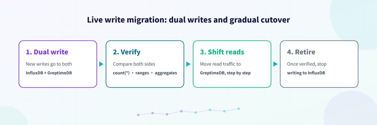
For a live migration, use dual writes or a gradual cutover: send new writes to both InfluxDB and GreptimeDB, compare count(*), time ranges, and key aggregation results, then shift read traffic to GreptimeDB step by step. Once everything checks out, stop writing to InfluxDB.

Live write migration: dual writes and gradual cutover

3. Migrate historical data

The most direct route for historical data is to keep using the InfluxDB line protocol. Nothing fancy here: as long as you can export the history as line protocol, you can import it through GreptimeDB's InfluxDB write API.

In this TSBS walkthrough, tsbs-iot-influx.gz is itself the historical data file. Importing it into GreptimeDB reuses the shell pattern from the official migration documentation:

export GREPTIME_HOST="localhost"
export GREPTIME_DB="public"

for file in ./tsbs-iot-parts/data.*; do
  curl -i --retry 3 \
    -X POST "http://${GREPTIME_HOST}:4000/v1/influxdb/write?db=${GREPTIME_DB}&precision=ns" \
    --data-binary @"${file}"
  sleep 1
done

If your historical data comes from a real InfluxDB instance rather than a TSBS-generated file, a few guidelines apply:

• For small datasets, re-export the data as line protocol from the application side or with a script, then import it through the GreptimeDB write API.

• For large datasets, export in batches by measurement and time range, keep individual batch files small, and record checkpoints so you can resume.

• For measurements with high-cardinality tags, confirm before importing that the primary key columns of the GreptimeDB table match your expectations; automatic table creation maps line protocol tags to primary key columns.

• After importing, verify at least the row count, time range, non-null field counts, and key aggregation queries for each measurement.

Common verification SQL:

SELECT
  count(*) AS row_count,
  min(greptime_timestamp) AS min_ts,
  max(greptime_timestamp) AS max_ts
FROM readings;

SELECT
  count(*) AS row_count,
  min(greptime_timestamp) AS min_ts,
  max(greptime_timestamp) AS max_ts
FROM diagnostics;

SELECT fleet, count(*) AS row_count
FROM readings
GROUP BY fleet
ORDER BY row_count DESC;

4. Migrate InfluxQL to GreptimeDB SQL

The TSBS InfluxDB IoT queries cover two kinds of workloads:

• Real-time status queries: things like the last location of a set of vehicles, low fuel, high load, or unusually long driving sessions.

• Analytical queries: aggregations by fleet, model, driver, day, or 10-minute window.

Before rewriting InfluxQL, map its concepts to their GreptimeDB SQL counterparts:

• An InfluxQL measurement corresponds to a GreptimeDB table name, such as readings or diagnostics.

• InfluxQL tags and fields are both columns in GreptimeDB; tags are usually also primary key columns.

• InfluxQL's time corresponds to greptime_timestamp in tables created automatically by line protocol ingestion.

• InfluxQL's GROUP BY time(10m), "name", "driver" becomes a GreptimeDB range query: avg(value) RANGE '10m' ... ALIGN '10m' BY (name, driver).

• For plain discrete bucketing, date_bin('10 minutes'::INTERVAL, greptime_timestamp) followed by GROUP BY also works.

• For selector queries like ORDER BY time DESC LIMIT 1, rewrite with row_number() OVER (...) to express "the latest point per group" explicitly.

• For state-change queries like difference() and elapsed(), rewriting with lag(), lead(), and CTEs is usually more readable.

The examples below migrate TSBS IoT InfluxQL queries to GreptimeDB SQL. They assume the TSBS data was written to GreptimeDB through line protocol, so the time column is greptime_timestamp.

AI tools handle most of this rewriting well. A simple prompt:

"I'm migrating from InfluxDB to GreptimeDB. Rewrite the following InfluxQL as SQL that GreptimeDB supports:

<InfluxQL to migrate>

Refer to at least these documents:

1. GreptimeDB's InfluxDB data model: https://docs.greptime.com/user-guide/ingest-data/for-iot/influxdb-line-protocol/#data-model

2. GreptimeDB's Range Query, optimized for time-series workloads: https://docs.greptime.com/reference/sql/range/

3. GreptimeDB's SQL reference: https://docs.greptime.com/reference/sql/overview/"

4.1 Vehicles with low average velocity in a 10-minute window

TSBS InfluxQL:

SELECT "name", "driver"
FROM (
  SELECT mean("velocity") AS mean_velocity
  FROM "readings"
  WHERE time > '2026-01-01T00:00:00Z' AND time <= '2026-01-01T00:10:00Z'
  GROUP BY time(10m), "name", "driver", "fleet"
  LIMIT 1
)
WHERE "fleet" = 'South' AND "mean_velocity" < 1
GROUP BY "name";

The core of this query is "aggregate velocity per vehicle over 10-minute windows." A GreptimeDB range query expresses those window semantics directly:

WITH velocity_by_window AS (
  SELECT
    greptime_timestamp,
    name,
    driver,
    avg(velocity) RANGE '10m' AS mean_velocity
  FROM readings
  WHERE greptime_timestamp > '2026-01-01T00:00:00Z'::TIMESTAMP
    AND greptime_timestamp <= '2026-01-01T00:10:00Z'::TIMESTAMP
    AND fleet = 'South'
  ALIGN '10m' BY (name, driver)
)
SELECT name, driver, greptime_timestamp, mean_velocity
FROM velocity_by_window
WHERE mean_velocity < 1;

Here RANGE '10m' means each aggregation window covers 10 minutes of data, ALIGN '10m' emits one aligned window result every 10 minutes, and BY (name, driver) corresponds to the tag grouping in InfluxQL.

4.2 Vehicles with long driving sessions within 4 hours

The TSBS long-driving query first computes average velocity over 10-minute windows, then counts the windows where the average exceeds 1. The InfluxQL structure looks roughly like this:

SELECT "name", "driver"
FROM (
  SELECT count(*) AS ten_min
  FROM (
    SELECT mean("velocity") AS mean_velocity
    FROM readings
    WHERE "fleet" = 'South'
      AND time > '2026-01-01T00:00:00Z'
      AND time <= '2026-01-01T04:00:00Z'
    GROUP BY time(10m), "name", "driver"
  )
  WHERE "mean_velocity" > 1
  GROUP BY "name", "driver"
)
WHERE ten_min > 22;

In GreptimeDB SQL, put the "10-minute driving window" in a CTE and aggregate again on top of it:

WITH driving_windows AS (
  SELECT
    greptime_timestamp,
    name,
    driver,
    avg(velocity) RANGE '10m' AS mean_velocity
  FROM readings
  WHERE fleet = 'South'
    AND greptime_timestamp > '2026-01-01T00:00:00Z'::TIMESTAMP
    AND greptime_timestamp <= '2026-01-01T04:00:00Z'::TIMESTAMP
  ALIGN '10m' BY (name, driver)
)
SELECT
  name,
  driver,
  count(*) AS driving_10m_windows
FROM driving_windows
WHERE mean_velocity > 1
GROUP BY name, driver
HAVING count(*) > 22;

The threshold 22 comes from the TSBS calculation: within the 4-hour span, each hour allows a 5-minute break, and converting the remaining driving time into 10-minute windows gives 22. The 24-hour version follows the same rewrite; just widen the time range to 24 hours and adjust the threshold to the corresponding window count.

4.3 Average daily driving duration

The TSBS daily driving duration query also starts with 10-minute window aggregation, then counts windows per day and divides by 6 to convert 10-minute windows into hours. The InfluxQL structure can be summarized as:

SELECT count("mv") / 6 AS "hours driven"
FROM (
  SELECT mean("velocity") AS "mv"
  FROM "readings"
  WHERE time > '2026-01-01T00:00:00Z'
    AND time < '2026-01-02T00:00:00Z'
  GROUP BY time(10m), "fleet", "name", "driver"
)
WHERE time > '2026-01-01T00:00:00Z'
  AND time < '2026-01-02T00:00:00Z'
GROUP BY time(1d), "fleet", "name", "driver";

GreptimeDB SQL:

WITH ten_minute_windows AS (
  SELECT
    greptime_timestamp,
    fleet,
    name,
    driver,
    avg(velocity) RANGE '10m' AS mean_velocity
  FROM readings
  WHERE greptime_timestamp > '2026-01-01T00:00:00Z'::TIMESTAMP
    AND greptime_timestamp < '2026-01-02T00:00:00Z'::TIMESTAMP
  ALIGN '10m' BY (fleet, name, driver)
),
daily_sessions AS (
  SELECT
    fleet,
    name,
    driver,
    date_bin('1 day'::INTERVAL, greptime_timestamp) AS day,
    count(*) / 6.0 AS hours_driven
  FROM ten_minute_windows
  WHERE mean_velocity > 1
  GROUP BY fleet, name, driver, day
)
SELECT
  fleet,
  name,
  driver,
  avg(hours_driven) AS avg_daily_hours
FROM daily_sessions
GROUP BY fleet, name, driver
ORDER BY fleet, name, driver;

This query shows a common migration pattern: the first layer is a range query that shapes raw points into 10-minute windows, and the second layer is plain SQL that rolls them up by day. For multi-stage aggregations like this, CTEs are easier to maintain than InfluxQL's nested subqueries.

Summary

A migration from InfluxDB to GreptimeDB splits into two tracks that can run in parallel:

• Writes and historical data take the InfluxDB line protocol compatibility path, getting data into GreptimeDB reliably first.

• Queries move from InfluxQL to SQL: measurements, tags, and fields become tables and columns, and GROUP BY time(...) becomes date_bin(...) or a GreptimeDB range query.

For typical time-series analytical workloads like TSBS IoT, GreptimeDB's SQL is often more direct than InfluxQL: window functions for latest points, lag()/lead() for state changes, date_bin() for fixed-window bucketing, and RANGE ... ALIGN ... BY ... FILL ... when you need step-aligned windows with gap filling. Don't migrate by syntax substitution alone; recover the business semantics first, then pick the clearest, most maintainable SQL that GreptimeDB offers.