What is Distributed Tracing

In today’s increasingly complex microservices architectures, distributed tracing has become a foundational pillar of observability. Tracing enables developers to pinpoint performance bottlenecks, understand system behaviors, and debug distributed systems effectively.

The concept was first systematically introduced in Google's seminal paper on the Dapper system, which later inspired the creation of Jaeger by Uber engineers. Today, Jaeger is a key project within the CNCF ecosystem.

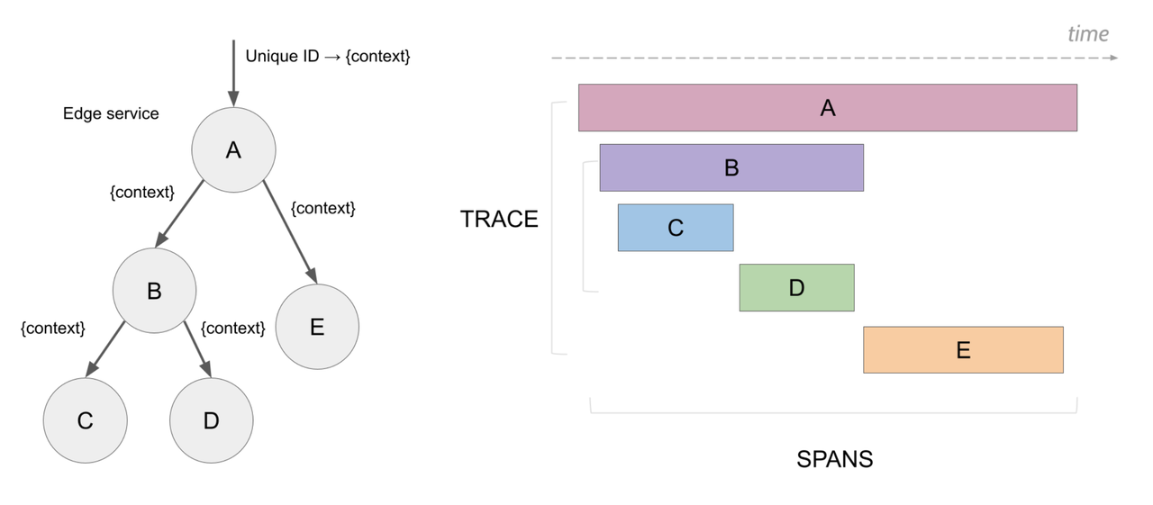
• Distributed tracing abstracts each end-to-end request across multiple services as a Trace. Each step within that request is represented as a Span, the atomic unit in tracing, annotated with metadata and uniquely identified by a span_id.
• A complete trace consists of multiple causally-related spans and is uniquely identified using a trace_id.

Refer from Jaeger :

（Figure 1: Data Model of Traces）

The OpenTelemetry community has established a canonical data model for traces, which has become the de facto industry standard. For example, a complete trace in JSON format may look like this:

{
  "resourceSpans": [
    {
      "resource": {
        "attributes": [
          {
            "key": "service.name",
            "value": {
              "stringValue": "my.service"
            }
          }
        ]
      },
      "scopeSpans": [
        {
          "scope": {
            "name": "my.library",
            "version": "1.0.0",
            "attributes": [
              {
                "key": "my.scope.attribute",
                "value": {
                  "stringValue": "some scope attribute"
                }
              }
            ]
          },
          "spans": [
            {
              "traceId": "5B8EFFF798038103D269B633813FC60C",
              "spanId": "EEE19B7EC3C1B174",
              "parentSpanId": "EEE19B7EC3C1B173",
              "name": "I'm a server span",
              "startTimeUnixNano": "1544712660000000000",
              "endTimeUnixNano": "1544712661000000000",
              "kind": 2,
              "attributes": [
                {
                  "key": "my.span.attr",
                  "value": {
                    "stringValue": "some value"
                  }
                }
              ]
            }
          ]
        }
      ]
    }
  ]
}

In essence, trace data can be viewed as structured logs. Many organizations still output traces via logging. Thus, a database optimized for log storage is well-positioned to handle trace data as well. Solutions like ClickHouse and Elasticsearch are often used for both logs and traces.

GreptimeDB has demonstrated strong performance in JSON-intensive workloads, as seen in benchmark results from JSONBench. Now, with support for OpenTelemetry Traces, GreptimeDB extends its observability capabilities to tracing.

The Challenges of Scalable Trace Storage and Querying

From our conversations with enterprise users, we've identified five key challenges when scaling trace data systems:

1. High-Volume Ingestion: Trace data scales with service complexity. At large organizations, billions of spans may be generated daily, requiring millions of spans per second to be ingested in real time.

2. Real-Time Query: Most trace queries target recent data. Historical data is typically aggregated into metrics. Therefore, high data freshness and low query latency are essential.

3. Cost-Efficient Long-Term Storage: Given the volume, trace data is expensive to store. Head- or tail-based sampling is commonly used to reduce volume, and most traces have short TTLs (e.g., 7 days).

4. Correlated Analysis: Users often want to pivot from a trace to related logs or metrics using the trace_id or other semantic keys. Rich correlation capabilities are vital for root cause analysis.

5. Aggregated Computation: Single traces provide limited insight. Aggregated traces are used to derive business-level metrics such as RED (Rate, Error, Duration) or service topologies.

GreptimeDB’s Native OpenTelemetry Support

Embrace the OpenTelemetry

GreptimeDB embraces the OpenTelemetry standard and acts as a fully OpenTelemetry-native observability database. For trace ingestion, GreptimeDB supports the native OpenTelemetry HTTP endpoint:

OTEL_EXPORTER_OTLP_TRACES_ENDPOINT="http://cluster.greptime:4000/v1/otlp/v1/traces"
OTEL_EXPORTER_OTLP_TRACES_HEADERS="x-greptime-pipeline-name=greptime_trace_v1"

These configurations allow applications instrumented with the OpenTelemetry SDK to export trace data directly into GreptimeDB.

Internally, GreptimeDB maps all trace data into a distributed table named opentelemetry_traces, partitioned by trace_id. By default, this table is sharded into 16 regions to distribute ingestion and query load. In the enterprise edition, region partitioning can scale dynamically based on ingestion pressure.

Map-type fields like attributes are flattened into individual columns during ingestion. This improves both storage compression and query performance. Key columns like trace_id and service_name use skipping indexes to accelerate filtering while minimizing indexing overhead.

More details can be found in our documentation.

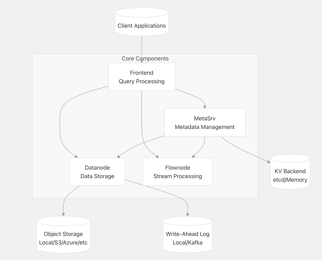
Separation of Compute and Storage: Low-Cost and Elastic

GreptimeDB’s architecture separates compute from storage. Data is persisted in cost-efficient object storage, while SSD-based cloud volumes are used for WALs and caching to ensure reliability and performance.

（Figure 2: Separation of Compute and Storage）

Traditional monolithic databases that tightly couple compute and storage—such as Elasticsearch and ClickHouse—often struggle to balance read/write performance with low storage costs and high elasticity.

GreptimeDB, by adopting a disaggregated compute-storage architecture, achieves:

• Cost-effective data storage: All trace data is stored in inexpensive object storage, significantly lowering overall storage costs in large-scale scenarios—potentially by several times—compared to traditional cloud disks. A rough comparison using AWS S3 and EBS (actual costs vary by usage and region): storing 10 PB of data in S3 (standard storage) costs about $210,000 per month, whereas storing the same volume in EBS (gp3 type) costs up to $820,000. Users can further migrate historical tracing data to colder object storage over time to retain long-term archives for auditing or other purposes.

• Elastic compute resources: By decoupling compute from storage, GreptimeDB enables elastic scaling of compute nodes based on trace data load. Since trace data typically exhibits a “write-heavy, read-light” pattern, the enterprise version of GreptimeDB supports read/write separation, allowing users to scale out write nodes independently. This ensures high-throughput ingest without affecting query performance, thanks to isolation of compute resources.

Lightweight Stream Engine for Continuous Aggregation

In trace data processing, aggregation is nearly always necessary, especially for deriving metrics from traces via stream processing—an industry-standard approach. Instead of requiring users to manage a complex external streaming system, GreptimeDB provides a built-in lightweight stream engine that continuously aggregates data.

Stream processing in GreptimeDB is abstracted as a Flownode, similar to Datanode, and can elastically scale based on workload. Users can define real-time Flow tasks using simple SQL. For example:

CREATE FLOW IF NOT EXISTS `opentelemetry_traces_spans_red_metrics_1m_aggregation`
SINK TO `opentelemetry_traces_spans_red_metrics_1m`
COMMENT 'Calculate RED metrics for each span in 1 minute time window.'
AS
SELECT
    `service_name`,
    `span_name`,
    `span_kind`,
    count(*) as `total_count`,
    sum(case when `span_status_code` = 'STATUS_CODE_ERROR' then 1 else 0 end) as `error_count`,
    avg(`duration_nano`) as `avg_latency_nano`,
    uddsketch_state(128, 0.01, "duration_nano") AS `latency_sketch`,
    date_bin('1 minutes'::INTERVAL, `timestamp`, '2025-05-17 00:00:00') as `time_window`
FROM `opentelemetry_traces`
GROUP BY `service_name`, `span_name`, `span_kind`, `time_window`;

This defines a Flow named opentelemetry_traces_spans_red_metrics_1m_aggregation, which computes RED metrics per span in 1-minute windows, outputting to a new metrics table. Interestingly, because GreptimeDB supports PromQL, these metrics can be queried using PromQL and integrated seamlessly into the Prometheus ecosystem.

In addition to RED metrics, service dependency analysis is another classic trace use case. In the Jaeger ecosystem, the spark-dependencies project uses Spark to analyze service relationships. In GreptimeDB, this can be done via a single Flow:

CREATE FLOW IF NOT EXISTS `opentelemetry_traces_dependencies_1h_aggregation`
SINK TO `opentelemetry_traces_dependencies_1h`
COMMENT 'Calculate dependencies between services in 1 hour time window.'
AS
SELECT
    `parent`.`service_name` AS `parent_service`,
    `child`.`service_name` AS `child_service`,
    COUNT(*) AS `call_count`,
    date_bin('1 hour'::INTERVAL, `parent`.`timestamp`, '2025-05-17 00:00:00') as `time_window`
FROM `opentelemetry_traces` AS `child`
JOIN `opentelemetry_traces` AS `parent` ON `child`.`parent_span_id` = `parent`.`span_id`
WHERE `parent`.`service_name` != `child`.`service_name`
GROUP BY `parent_service`, `child_service`, `time_window`;

This aggregates call counts between services over one-hour intervals, making service topology computation much simpler. More advanced topology computations will be supported in the future.

Unified Observability Data Storage

As mentioned earlier, tracing is far more valuable when correlated with logs and metrics. In GreptimeDB, users can store logs, metrics, and trace data in a single unified observability store, enabling powerful relational analysis via SQL. For example, based on shared fields like trace_id or service_name, users can:

• Perform simplified correlation analysis: The following SQL retrieves a full request context—including trace, log, and metric data—in a single query:

SELECT
    t.trace_id,
    t.span_id,
    t.span_name,
    t.duration_nano,
    t.status,
    t.service_name,
    l.timestamp,
    l.level,
    l.message,
    m.cpu,
    m.memory
FROM
    traces t
JOIN
    logs l ON t.trace_id = l.trace_id
JOIN
    metrics m ON t.service_name = m.service_name
WHERE
    t.trace_id = '4d6c62efe6be73c9c9f86e54b9b527e4'
ORDER BY
    l.timestamp;

This query reveals the relevant logs and system metrics associated with a specific trace, giving developers deep visibility into system behavior.

• Achieve better performance and simplicity: Since all observability data is stored together, queries are more efficient, data governance is simplified, and the overall architecture becomes cleaner and easier to manage.

SQL + Jaeger API Support

GreptimeDB supports SQL natively, allowing users to query trace data without learning a new DSL. Furthermore, since Jaeger is one of the most popular distributed tracing systems, GreptimeDB also implements most of the Jaeger query APIs. In fact, because Jaeger lacks its own query language, GreptimeDB maps Jaeger API calls directly to SQL equivalents—making compatibility relatively straightforward.

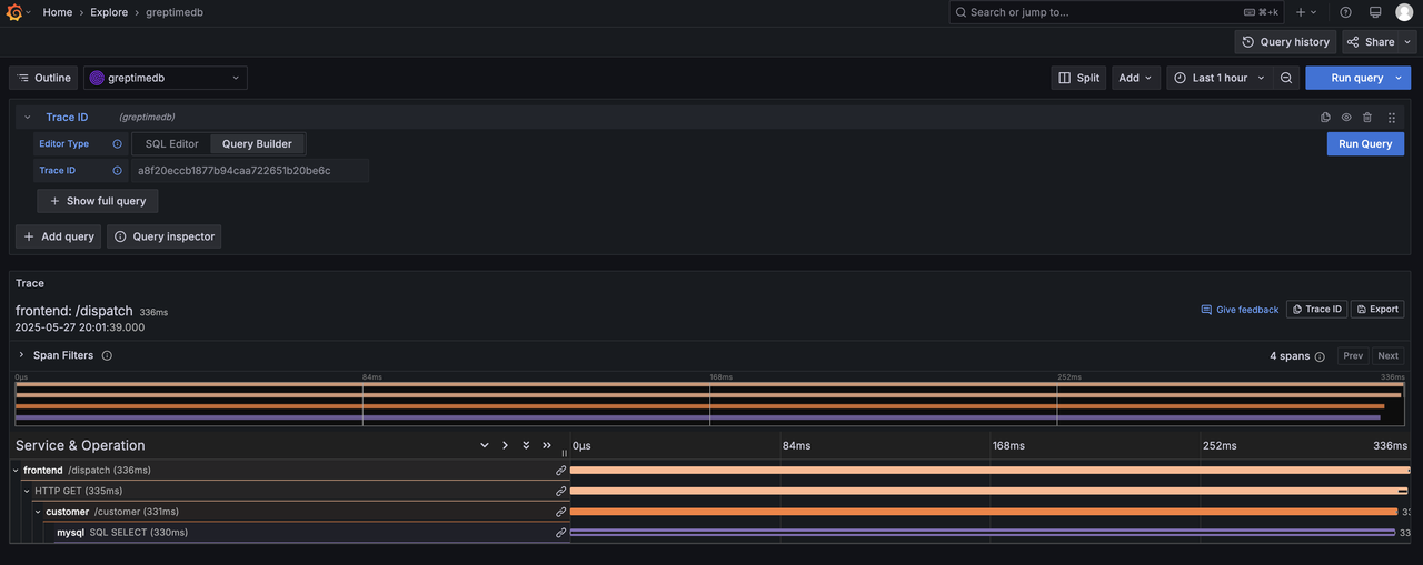
Thanks to this Jaeger API compatibility, users can continue to use familiar tools like Grafana’s Jaeger plugin or the Jaeger UI for querying and visualization.

Grafana Plugin Support

To further enrich the Grafana ecosystem, we've open-sourced the GreptimeDB Data Source plugin. Following the integration guide, users can visualize trace data and even configure Trace ID-based deep linking into logs:

（Figure 3: Grafana Plugin Support）

Roadmap

Support for tracing in GreptimeDB is evolving rapidly. Our goal is to meet user needs across different scales with exceptional performance and ease of use. In the near future, we will focus on:

• Higher ingest throughput: We're developing higher-throughput write paths to support real-time ingestion of even larger-scale trace data for enterprise use.
• Built-in Flow templates and trace-specific SQL functions: To lower the entry barrier, we’ll bundle commonly used Flow tasks (like RED metrics) and provide native SQL functions tailored for trace queries, making querying easier out of the box.
• TraceBench project: Unlike logging, tracing lacks standardized benchmarks. We plan to introduce TraceBench, a tracing-focused benchmark suite built on top of JSONBench, to help the community with more informed technical evaluations.